Decoding Gene Set Variation Analysis
Characterising biological pathways from gene expression data
Gene Set Variation analysis is a technique for characterising pathways or signature summaries from a gene expression dataset. GSVA builds on top of Gene Set Enrichment analysis where a set of genes is characterised between two condition groups defined in the sample. GSEA (Gene set enrichment analysis) works on how genes are behaving differently between the two groups defined. Do you need to understand GSEA to go ahead with this? Absolutely not. The only thing you can pick up from GSEA is that it uses a very basic concept called the ‘running sum’ which I will explain here as well.
Why do I even need GSVA?
Simply because GSEA relies on phenotypic data and samples are looked at in a way that two groups of samples whose phenotype I already know have to be compared. What if I want to study my samples for the enrichment of a pathway without relying on phenotypic information. What if I want to ask, how is this pathway or gene signature behaving in this sample? Gene Set Variation analysis can help me out here!
Let’s just get into it because you’re (probably) more interested in knowing how it works. I first explain how GSVA works on the surface by applying it on an actual dataset of pancreatic cancer and then we go into the depth of it by looking at what does it do to an extremely small dataset. You may skip to the latter if you are already somewhat familiar with what GSVA is on a broad level.
Steps in GSVA
Fitting the data to a model
The first step in GSVA is estimating the RNASeq or microarray data with a model. Why use a model when you have the actual data? Because models are clean, free from extremities, and easy to operate on.
RNAseq data is modelled by a Poisson distribution, and while some would argue that it is actually negative binomial and they are not wrong but let’s just consider it to be Poisson for now. Very briefly, think of an experiment where you try to sprinkle chocolate chips on a cookie from a very large distance — the number of chocolate chips landing on a cookie can be 0….any possible number. If you try to estimate the number of chocolate chips on a cookie it follows a Poisson distribution. In a similar manner, in an RNASeq experiment you are trying to get how many reads among all reads fall within the transcript of a gene. The transcripts are your chocolate chips and the gene is your cookie. That is why the counts of a gene follows a Poisson process.
In the case of microarray data, the intensity of each gene is modelled as Gaussian or normal distribution. Note that in the case of log transformed RNA Seq data, or any other continuous counts it is good to estimate it from a Gaussian distribution and when the data has integer values (for eg. raw counts) a Poisson kernel should be used to estimate it
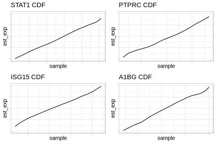
The cumulative density function is estimated for every gene using all samples from the above distributions. In simpler terms a CDF value is assigned to each gene in each sample.
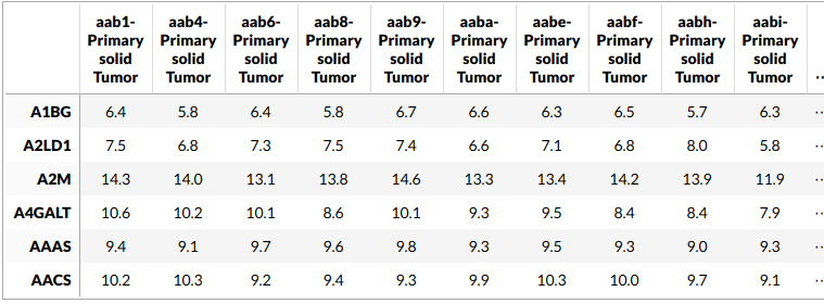
This is how our RNA expression data looks like. We have ~15,000 genes in 183 samples.
 Let’s look at the CDFs of the fitted distributions for some of the genes.
 The CDF has been estimated for each gene. The next step is to rank each each gene for every sample. It will be later clarified why we rank each gene in every sample. Note that these ranks are used to calculate the GSVA scores.
Defining gene sets
It’s no surprise that we need a gene set to do GSVA. These gene sets may come from anywhere — a pathway you might be interested in, a gene signature you discovered in an experiment or a signature you found out from a paper written 10 years ago. Say we want to study two signatures : -
- type 1 Interferon signature — This signature consists of 25 genes.
- type 1 Interferon stimulated genes — This signature consists of 125 genes.
Calculating GSVA scores — K-S statistic and empirical distributions
Now that we have our ranked genes and our gene sets the next step is calculating the GSVA score. This is done using the Klimigrov random walk statistic.
The K-S statistic is a method of judging if an empirical distribution is similar to another distribution. In our case we have to define two distributions, a distribution for the genes which lie in the geneset and another distribution of the genes which do not lie in the gene set. Our question is simple : How much do the genes in our gene set vary relative to the genes not in the gene set?
What is an empirical CDF? An empirical CDF is just a way of estimating the true CDF of a population from a sample and finding the empirical CDF is done with the use of order statistics or rank of each observation. Very briefly, for a sample of observations x1,x2,x3…xn drawn from an unknown distribution the empirical cumulative distribution function at any point x is the proportion of observations with value less than or equal to x. Don’t confuse this with the CDF we found out earlier. This CDF is for a combination of genes and different from the one estimated earlier using the whole data.
The distributions for both the genes in the gene set and the genes not in the gene set for a particular sample are calculated and the difference in these two distributions is the K-S statistic. How all this is done will be shown in the example later.
GSVA scores for our samples
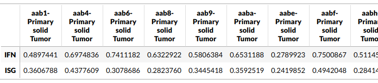 Now you have the the GSVA scores for both the signatures for every sample. What is this score, how was it calculated and what does it even tell us? A stimulated example would clarify this better.
Example
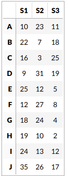
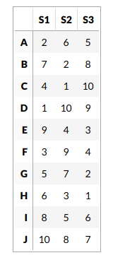
For our sanity let’s consider a dataset which has 3 samples and 10 genes.
Estimating CDF for every gene and finding ranks
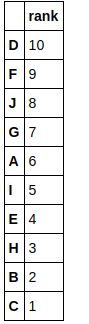
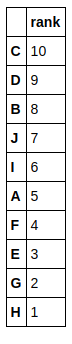
This step is skipped here and we assume that we have calculated CDFs already. This is because calculating CDFs from such a small data would give a poor estimation and defeat our purpose of understanding GSVA with an example. So let’s assume we have estimated the distribution for every gene using a Gaussian kernel and ranked the genes for every sample. Here are the ranks.
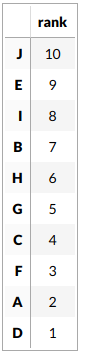
Let us define our gene set us consisting of the genes B, E and H
Let’s find GSVA scores for each sample separately. Note that the GSVA score calculation for a sample is still dependent on every sample as the CDF of each gene is estimated using all the samples.
Sample 1
The idea of random walk in this context is to iterate over every gene one by one, and check if it is in the gene set. The order of this iteration is defined by the ranking of genes for a sample. So genes are iterated over from the most positively expressed gene to the most negatively expressed genes. Let us define this order for sample 1:
Random walking and running sum
A random walk is about calculating a running sum. This is done by iterating over every gene, and checking if it lies or does not lie in the geneset.
We do two random walks here. One for genes lying in the gene set and one for genes not in the gene set. For the first case, we iterate over each gene and check if it lies in the gene set.
- If it does, add the rank of the gene to the running sum.
-
If it does not do not do anything and keep the running sum as is. For genes lying outside the gene set it is done by iterating over every gene.
- If the gene does not lie in the gene set, add 1 to the running sum
- If the gene lies in the gene set, do nothing and keep the running sum as is. Notice how while calculating the running sum for genes that do not lie in the gene set we do not add their ranks but just add 1 to the running sum. This gives us the intuition that we want to give weightage to genes lying in the gene set and we are more concerned with that.
Running sum for genes in gene set
This is how a random walk looks like for genes lying in the gene set.
Notice how the ‘RISE’ is greater for gene ‘E’ and the magnitude of the RISE for genes not in the gene set(genes ‘B’ and ‘H’) keeps on decreasing. This is because the rank of gene ‘E’ is higher. In other words we are rising proportional to how much a gene is expressed.
Running sum for genes not in gene set
After finding the running sums for genes lying in the gene sets we do a similar exercise for genes not present in the gene set. Notice how the ‘RISE’ is by an equal amount each time.
This is how a random walk looks like for the genes not in the gene set.
GSVA score for Sample 1
After I have found out both of these random walks, I need to quantify how different they are. One way of doing this is to take the maximum deviations between these two. The deviations between the two could be both in the positive and negative directions. I consider the maximum deviations in both the directions and take their difference to be the GSVA score.
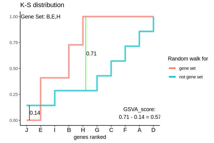
The GSVA score comes out to be 0.57. Which is highly positive and indicates that genes in the genes are positively enriched as compared to genes not in the gene set.
Sample 2
Note that B, E and H genes are now all among the lowly ranked genes
Running sum for genes in gene set
This is how the random walk looks like for genes lying in the gene set.
Running sum for genes not in gene set
This is how the random walk looks for the distribution of genes not lying in the gene set.
GSVA score for Sample 2
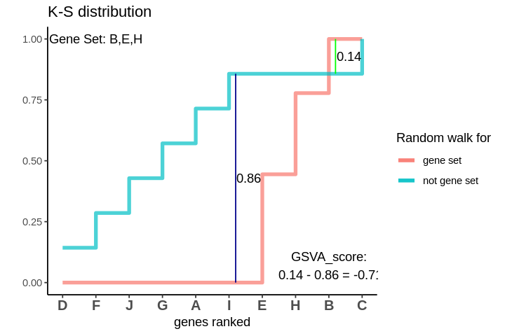
The GSVA score comes out to be -0.71. Which is highly negative and indicates that genes in the genes are negatively enriched as compared to genes not in the gene set.
Sample 3
Note that B is one of the higher ranked genes and E and H genes among the lowly ranked genes. Can you guess what the GSVA score would come out to be for such a case? Perhaps, it will be close to 0 ? Let’s see.
Running sum for genes in gene set
This is how the random walk looks like for genes lying in the gene set.
Running sum for genes not in gene set
This is how the random walk looks for the distribution of genes not lying in the gene set.
GSVA score for Sample 3
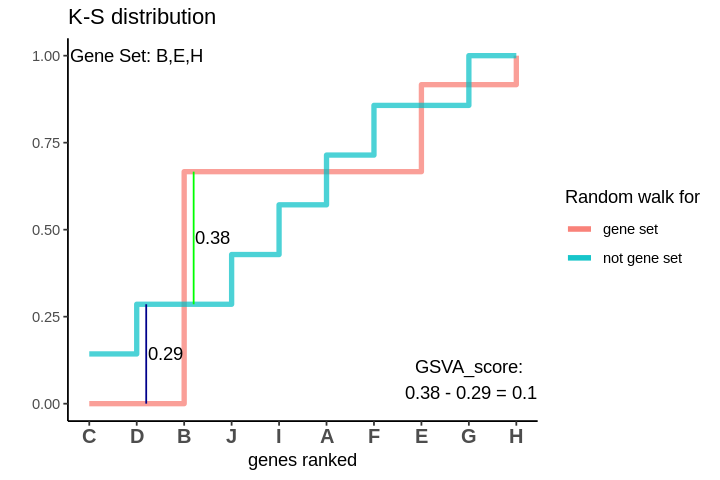
The distributions are intermingling. The GSVA score comes out to be 0.1 which is very close to 0. This means that the genes are neither positively or negatively enriched as compared to genes not in the gene set. So, if the some genes of the gene set lie in the higher ranks and some lie in the lower ranks their effect is cancelled out and the GSVA score comes out to be close to 0.
Conclusion
In conclusion the GSVA is a key method of quantifying enrichment in pathways and signatures on a sample by sample basis. It gives a very clever method which is based on the simple intuition that a gene set’s enrichment in a sample will depend on where the genes lie when we rank all the genes and look for the positions of the gene set’s genes in the ranked list.