How many children in a family? Depends on who you ask
In 2017, sociologist Elizabeth Wrigley-Field posed the following puzzle in this article:
To understand this phenomenon we need to understand how length-biased sampling works and how the sampling method can influence an estimate of a statistic. I will attempt to explain this from a probabilistic point of view by drawing samples and calculating the expected values for the number of children in a family. Before jumping onto the probablistic view, let’s understand intuitively how the sample collection method influences an estimate.
Pauline asks parents; Chris asks children
Let’s assume that we need to estimate the average family size of a neighbourhood at a particular point of time i.e. we assume that the children in a family are not becoming parents, and that a ‘family’ consists of parents and children (and possibly no children) only. To estimate the size of the family, we get two surveyors - Pauline and Chris. Pauline decides to go to each home and talk to the parent(s)whereas Chris stalks the children in the neighbourhood park every day. They both ask the same question:
How many children are there in your family?
After a week, they come back with their collected datasets. The first question we can ask is– Whose dataset has more rows?
Clearly, Chris has a much bigger dataset because he has the response of each child of the neighbourhood while Pauline has the response of each parent only. As every parent is expected to have zero or more children, Chris will have more responses. Essentially, both have collected the same dataset but represented differently. It’s possible to reconstruct Chris’ dataset from Pauline’s dataset and vice-versa.
| Pauline's dataset | Chris' dataset | ||||||||||||||||||||||||||||||||||||||||||
|---|---|---|---|---|---|---|---|---|---|---|---|---|---|---|---|---|---|---|---|---|---|---|---|---|---|---|---|---|---|---|---|---|---|---|---|---|---|---|---|---|---|---|---|
|
|
Now both Pauline and Chris come up with an estimate for the average number of children in a family in the area.
Chris's average = $\dfrac{4.3 + 3.4 + 1.1 + 2.2 +2.2+2.2}{12}$ = 3.08
The two averages are different but answering the same question. This simply says that for an “average kid” in a neighbourhood the family size is bigger than the family size for an “average parent”. As each kid is expected to come from a family of one or more than one children, the children’s responses are weighted by their family size, with each family size being greater than or equal to one. This is why sampling using children will always lead to a larger family size. This is how the length of the sample(longer in Chris’ case) biases the estimate. But wait, there’s more…
Can we foresee this with expected values?
Now, let’s try to understand this phenomenon from a probabalistic point of view. In a population study, the estimate of the statistic “average number of average children in a family in this neighbourhood” is random. Another way of thinking about it is to ask if we picked a random family or child in the neighborhood, what would be the number of children in that family? This is random (as we’re choosing randomly). We can denote this using a random variable, and calculate probabilities of the random variable taking on different values.
We denote $n_k$ to be the number of families in our population with exactly $k$ children. ($k \in \mathbb{N}\cup{0}$). This also means that there are $\sum_{k=0}^{\infty} k n_k$ children in total.
We then define two random variables:
- $F$: Number of children in the family of a family selected randomly.
- $C$: Number of children in the family of a child selected randomly.
As we don’t have any data about the neighbourhood, we can assume that both $F, C \in \mathbb{N}\cup {0}$, although a family with more than 10 children requires a stretch of the imagination. $F$ and $C$ are discrete random variables with distributions given by
\[\begin{align*} P(F=k) = \dfrac{n_k}{\sum\limits_{k=0}^\infty n_k} = \frac{n_k}{m_0},\\ P(C=k) = \dfrac{k n_k}{\sum\limits_{k=0}^\infty k n_k} = \frac{k n_k}{m_1}, \end{align*}\]where we have defined $m_j = \sum_{k=0}^\infty k^j n_k$.
These values arise from the fact that there are $n_k$ favourable events for ${F=k}$ and $kn_k$ favorable events for ${C=k}$, with the total number of events given by the denominator in each case.
Now we can calculate the expected values of $F$ and $C$,
\[\begin{align*} E(F) = \sum_{k=0}^{\infty} k P(F=k) = \sum_{k=0}^{\infty} k \frac{n_k}{m_0} = \frac{m_1}{m_0},\\ E(C) = \sum_{k=0}^{\infty} k P(C=k) = \sum_{k=0}^{\infty} \frac{k^2 n_k}{m_1} = \frac{m_2}{m_1}. \end{align*}\]Now, $\dfrac{m_2}{m_1} \geq \dfrac{m_1}{m_0}$,
Proof
We will prove this by induction. It's clearly true for $q=1$, let's assume it's true for $q$, i.e. $$ \begin{align} &\frac{m_2^q}{m_1^q} - \frac{m_1^q}{m_0^q} = \frac {\sum\limits_{k=0}^q k^2 n_k}{\sum\limits_{k=0}^q k n_k} \geq \frac{\sum\limits_{k=0}^q k n_k}{\sum\limits_{k=0}^q n_k}\\ \implies & m_2^q m_0^q - (m_1^q)^2 \geq 0. \end{align} $$ Now for $q+1$, and using the above expression, $$ \begin{align*} &\frac{m_2^{q+1}}{m_1^{q+1}} - \frac{m_1^{q+1}}{m_0^{q+1}} = \frac{m_2^q + (q+1)^2n_{q+1}}{m_1^q + (q+1)n_{q+1}} - \frac{m_1^q + (q+1)n_{q+1}}{m_0^q + n_{q+1}}\\ & = \frac{m_2^q m_0^q + (q+1)^2 n_{q+1}m_0^q + m_2^q n_{q+1} + (q+1)^2 n_{q+1}^2 - (m_1^q)^2 - (q+1)^2 n_{q+1}^2 - 2m_1^q (q+1)n_{q+1}}{m_1^{q+1} m_0^{q+1}}\\ & \geq \frac{(q+1)^2 n_{q+1}m_0^q + m_2^q n_{q+1} - 2m_1^q (q+1)n_{q+1}}{m_1^{q+1} m_0^{q+1}}\\ & = \frac{n_{q+1} [m^2_q + (q+1)^2 m_0^q - 2m_1^q(q+1)]}{m_1^{q+1} m_0^{q+1}}. \end{align*} $$ In the numerator of the above expression, coefficient of $n_k$ for $k=0...q$, is given by $$ k^2 + (q+1) [(q+1) - 2k], $$ which is positive for all $k = 0...q$ and $q \geq 2 $. Therefore, we get, $$ \begin{align*} \frac{m_2^{q+1}}{m_1^{q+1}} - \frac{m_1^{q+1}}{m_0^{q+1}} \geq 0. \end{align*} $$
So the expected value for the number of children in the family of a child when the child is chosen randomly is greater than the number of children when the family is chosen randomly. This explains the effect seen above using averages, but with expected values of random variables.
But how does this tie back to the Great Depression and the Baby Boom?
So far, we know that
\[\begin{align*} E(F_{\text{depression}}) < E(C_{\text{depression}})\\ E(F_{\text{boom}}) < E(C_{\text{boom}})\\ \end{align*}\]This just means that for both eras, the expected family size while sampling with children will be greater than the expected family size while sampling with families.
But can we compare expected values across different eras? Making a comparison of expected values will not make much sense without actual values. In general, we now know that during the Great Depression, families were either too large or too big, and during the Baby Boom family sizes were more uniformly distributed. In both cases, asking children would lead to a larger family size, but the Great Depression samples would have this effect pronounced more than the Baby Boom. Why? Because the children samples weigh each sample by the family size, and because of this large family sizes increase those weights more, thereby increasing the expected value. During the Baby Boom, family sizes were more uniform, so the effect of this weighting is not pronounced. Therefore, we may see the effect:
\[\begin{align*} E(F_{\text{depression}}) < E(F_{\text{boom}})\\ E(C_{\text{boom}}) < E(C_{\text{depression}})\\ \end{align*}\]With this it would be possible to arrange the 4 quantities in an order:
$E(F_{\text{depression}}) < E(F_{\text{boom}}) < E(C_{\text{boom}}) < E(C_{\text{depression}})$
This would perfectly explain the puzzle. As the cross-era relation can’t be seen arithmetically, let’s simulate the samples from the two eras.
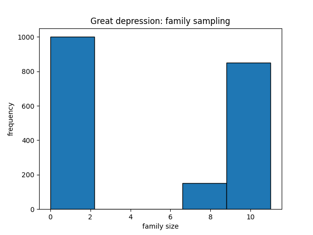
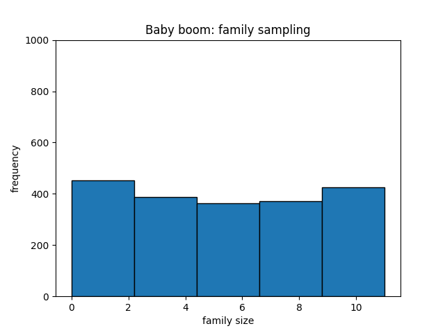
We can consider the example shown in the figure, where the frequency histogram is for a sample generated from the Great Depression and the Baby Boom. In both cases, the sample size is around 2000 families. It can be seen that the during the Great Depression, family sizes are on the extremes and during the Baby Boom, they are more uniformly distributed. This captures our assumption about the population during the two eras.
The above figures show the frequency distributions when the samples are generated by asking a parent in the family but what happens when the samples are generated by asking the children. Figure shows how the two distributions change. In both eras, the child sample histogram is majorly skewed to the right. This is expected because children from large families will be overrepresented in the sample. We can also calculate the expected values for the four random variables. They are plotted in the histograms with dotted lines.
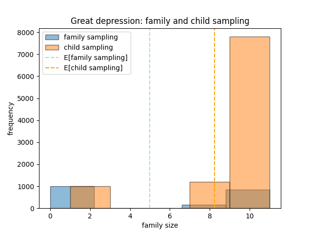
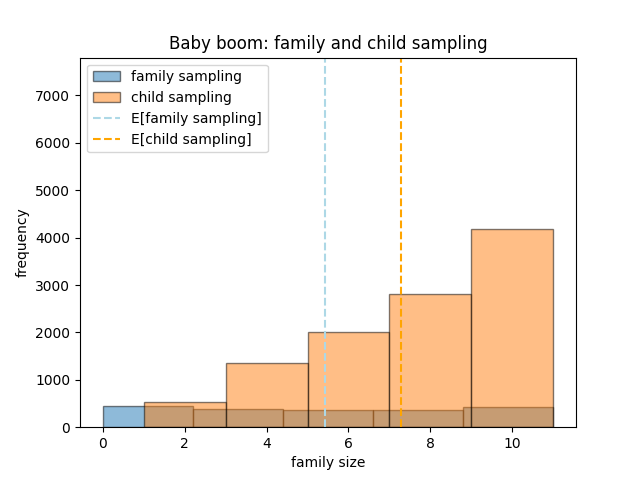
It is clear from the two figures, that parents had smaller family sizes on average during the Great Depression as compared to the Baby Boom (blue dotted line), whereas the average child came from a larger family during the Great Depression as compared to the Baby Boom (orange dotted line). The simulation agrees with our initial hypothesis and explains the effect of length-biased sampling.
There are other examples where length-biased sampling shows up. Some examples are given in the article. It just goes to show that estimating a population statistic might seem simple at first but it all depends on who you ask.
References:
- K. Blitzstein, J., & Hwang, J. (2019). Introduction to Probability Second Edition. https://drive.google.com/file/d/1VmkAAGOYCTORq1wxSQqy255qLJjTNvBI/view
- (1970). In Edge.org. https://www.edge.org/response-detail/27022
Code for the sampling and plots is available here.